Using Conditional Formatting When Building Models

All—wanted to formally walk through how to use conditional formatting inside Google Sheets when building models. Super simple but extremely powerful once you start applying it the right way.

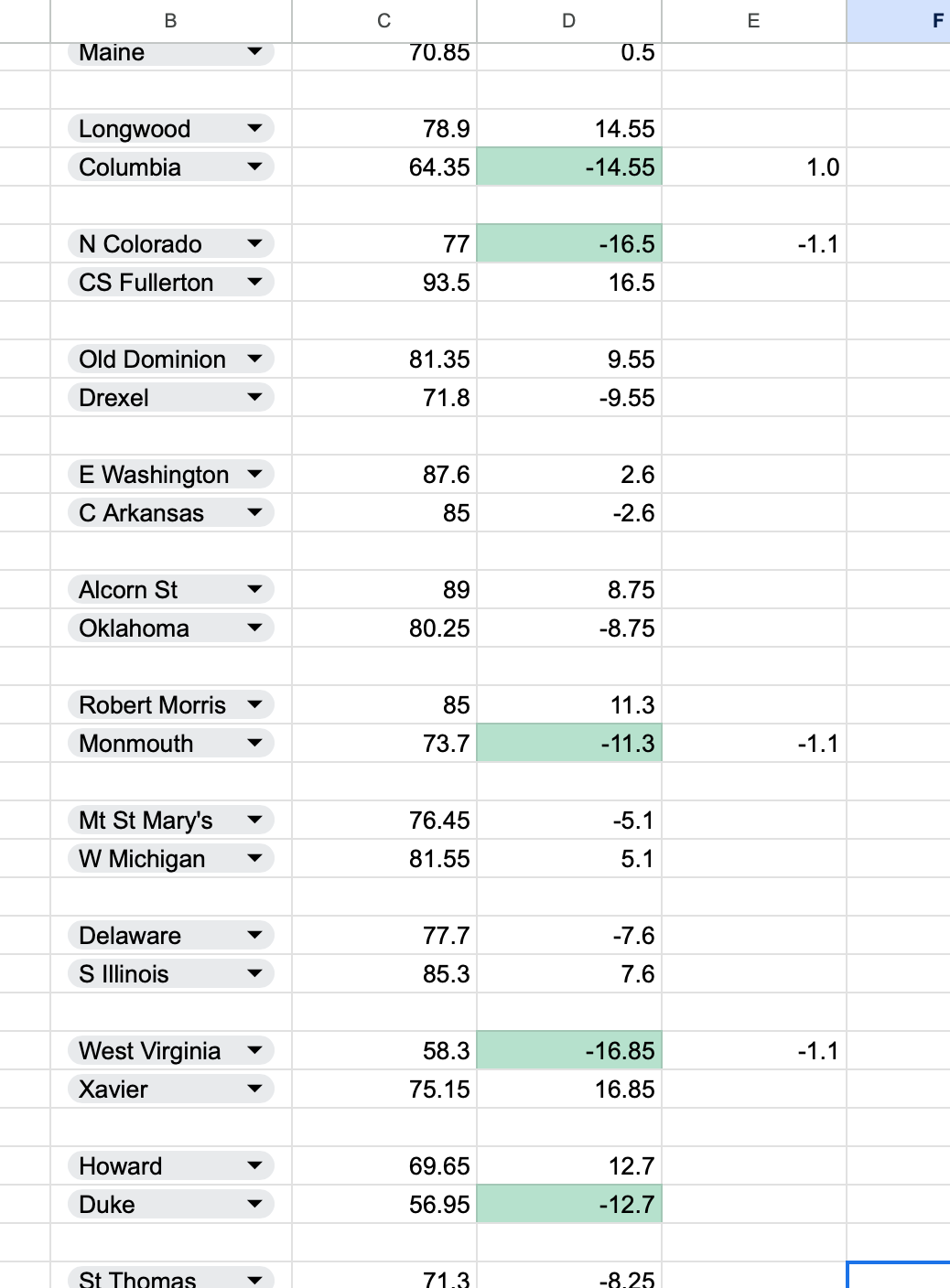
Let’s use the NCAAB model as the example.

In this model, we only look to play double-digit favorites based on our line. Instead of manually scanning for those numbers, conditional formatting lets Google Sheets highlight them for you automatically.

Step 1 — Select the Column

Click the column that contains your model lines. This is the data you want Google Sheets to read.

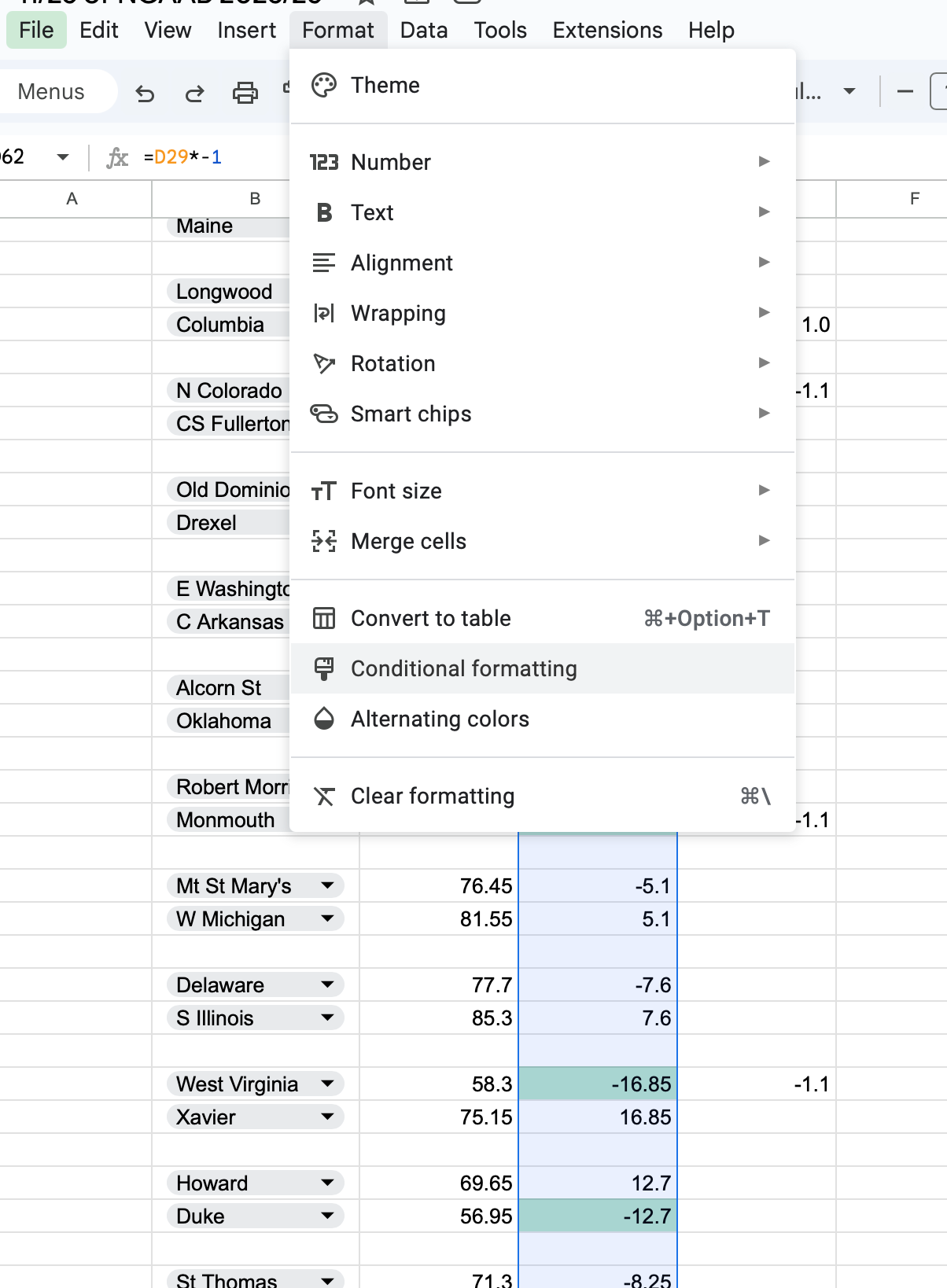
Step 2 — Open Conditional Formatting

Go to Format → Conditional Formatting.
A panel will pop up on the right side of the screen.

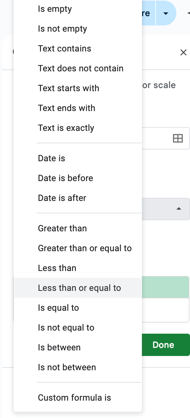
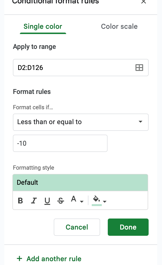
Step 3 — Tell Google Sheets What to Highlight

This is where you set the rule.

For the NCAAB model, we want to highlight double-digit favorites, so we use:

• Format cells if… → Less than or equal to -10

• 

Step 4 — Pick Your Color

Choose whatever highlight color you want for these plays.
I normally pick something bold so it pops immediately.

Custom Rules

You aren’t limited to just favorites.
You can customize conditional formatting to highlight:

• A differential between two numbers

• A margin %

• Any model trigger you use

• Anything that meets a condition inside your sheet

Once you understand this tool, you can automate a ton of the visual work inside your models.